

QPE (Quantitative Precipitation Estimates)
|
Quantitative precipitation estimates (QPE) refers to the analysis
of ground precipitation at locations or over a region of interest.
SWIRLS provides several methods to compute QPE:
|
|
Radar QPE is a real-time calibration approach for obtaining
rainfall rate through the Z-R relation Z=aR^b.
The coefficients a and b can be either
static based on climatological values, or dynamically
calibrated.
|
|
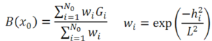
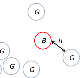
Barnes analysis interpolates data at grids from discrete rain
gauge data with Gaussian weighting based on distance between
data and estimation point:
|
|
|
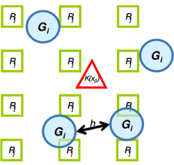
Co-kriging analysis is a geostatistical technique to derive
an optimal estimate of rainfall using both rain gauge and
radar reflectivity data. While computationally intensive,
co-kriging provides a sophisticated approach to estimate
rainfall amount taking into account the error characteristics
of rain gauge and radar measurements and their spatial
correlation.
|
Quality Control on Observations
|
The weather radars and raingauges are maintained with regular calibration to ensure high data quality for input to the nowcasting systems. Automatic raingauge data are not only fundamental in quantitative rainfall analysis but also used as the ground truth in warning operation and forecast validation. Quality control is necessary before the data can be used quantitatively due to systematic and random errors. Substantial random errors and unreasonably small or false zero values can hamper accuracy of the analysis of precipitation and effective monitoring of heavy rain.
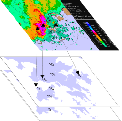
To address the issue, SWIRLS incorporates a real-time rainfall data quality-control scheme based on co-kriging analysis when blending radar and raingauge data to generate the quantitative precipitation estimate (QPE). As a basis of the quality-control scheme, the co-kriging rainfall analysis was shown through a verification exercise to be superior to those obtained by the Barnes analysis and ordinary kriging of raingauge data. An example is illustrated below. Details of the algorithm are described in the paper Development of an operational rainfall data quality-control scheme based on radar-raingauge co-kriging analysis
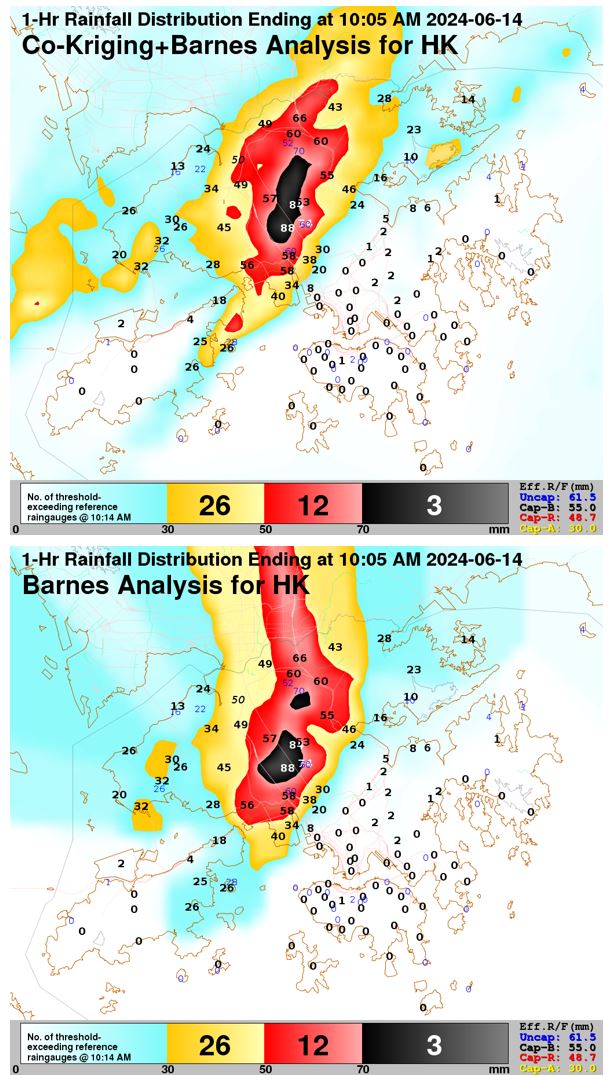
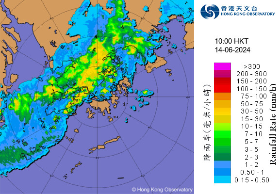
An example of co-kriging rainfall analysis and raingauge data quality-control valid at 10:05H on 14 June 2024 (top), along with the rainfall isohyet map based on the Barnes analysis method with only raingauge data (middle). A radar image at 10:00H (bottom) revealed significant rainfall over of territory of Hong Kong.
|
QPF (Quantitative Precipitation Forecasts)
|
Quantitative precipitation forecast (QPF) is the prediction of the
amount of rainfall that a particular area is expected to receive.
SWIRLS currently uses the advection-based model where QPF is
calculated through the following steps:
|
|
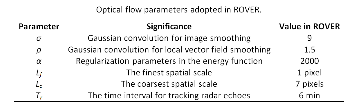
"Real-time Optical flow by Variational methods for Echoes of Radar
(ROVER)" is a real-time variational optical flow scheme, which
adopts 1) a pre-processing step to enhance radar reflectivity images;
and 2) a real-time variational optical flow technique.
1. Pre-processing step
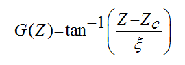
In ROVER, the reflectivity fields are enhanced by transforming the
gridded value with the following function:
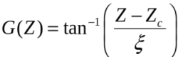 where Zc and ξ control the point of inflection and its sharpness.
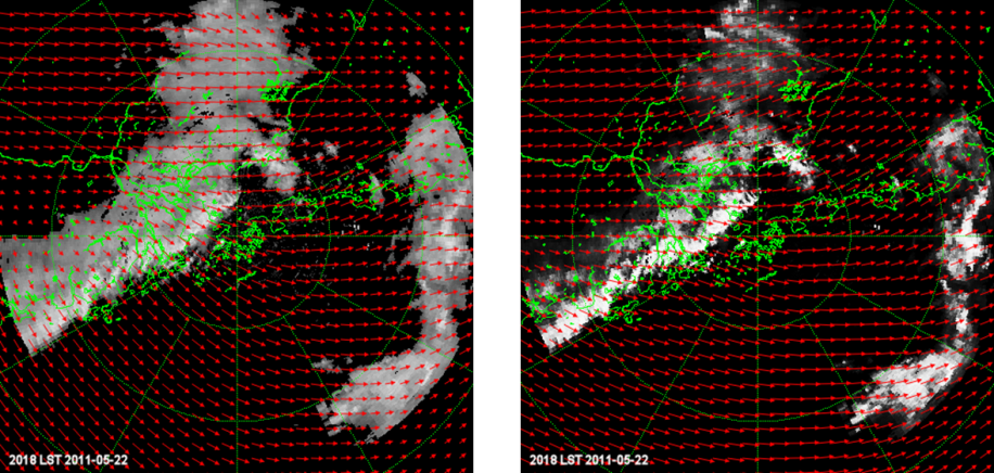
Figure 1. Original (left) and Enhanced (right) reflectivity map
2. Real-time variational optical flow technique
To generate the motion field, SWIRLS adopts the open source codes titled
"VarFlow" (Harmat, 2014), developed based on the algorithm proposed in
Bruhn et al. (2003).
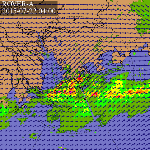
Figure 2. Motion field with arrows indicating motion vectors
|
|
After retrieval of the motion field, radar echoes are advected
with backward semi-Lagrangian advection scheme.
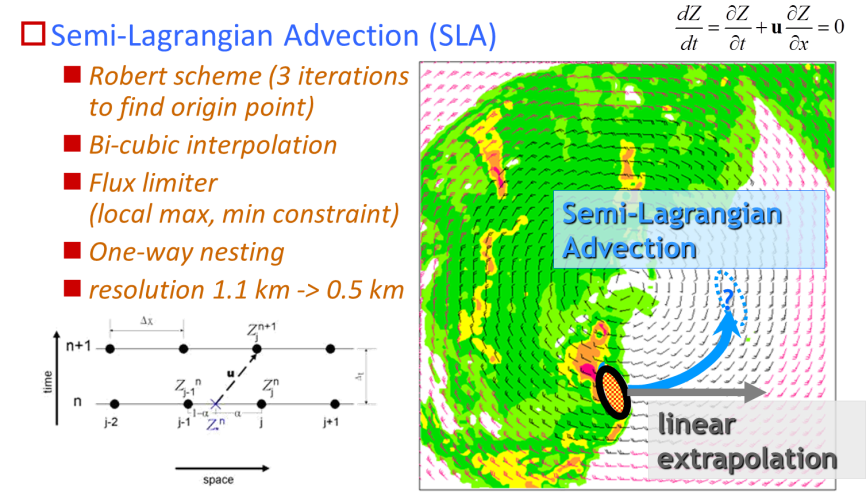
Figure 3. Semi-Lagrangian Advection scheme adopted in SWIRLS
|
|
Using Z-R relationship with static or dynamically calibrated
parameters, radar reflectivity data are converted and aggregated
to rainfall intensity data, such as hourly rainfall, which in
turn are used by downstream applications to generate user
products.
|
|
|
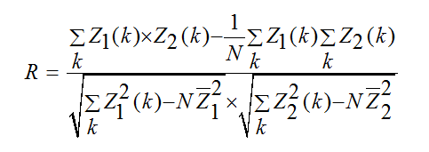
"Tracking Radar Echoes by Correlation (TREC)" essentially compares two successive radar reflectivity images and from which identifies a motion vector for each divided block of pixels through maximizing the correlation coefficient R, defined as follows:
|
|
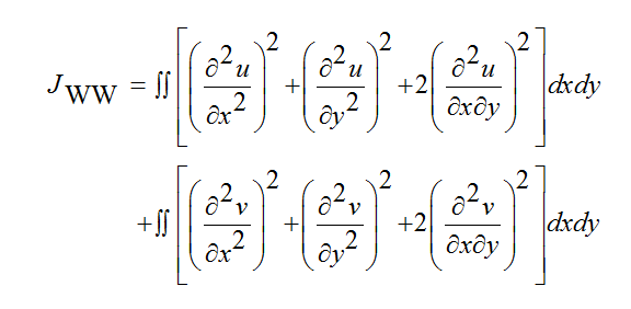
A radar echo tracking method utilizing variational optical flow technique, named as "Multi-scale Optical-flow by Variational Analysis (MOVA)", was developed in 2009.
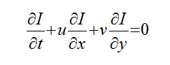
Defined as the apparent motion of brightness patterns in an image, optical flow would ideally equalize motion field barring lighting changes. Assuming that the brightness of a point of an object would remain unchanged along its path (i.e., "brightness constancy assumption"), the optical flow can be derived by solving the optical flow constraint (OFC) below:
|
|
While MOVA achieved improved overall performance over TREC, it has also been observed in operation that MOVA has a tendency to underestimate the speed of echo motion vectors, in particular at large scale, due to sub-optimal retrieval of echo motion in the minimization procedure. As a result, excessive rainfall was forecast at times. With a view to addressing the issue, another variational optical flow scheme, named as "Real-time Optical flow by Variational methods for Echoes of Radar (ROVER)", was used instead. In brief, ROVER is similar to MOVA but with two major enhancements: (1) having a pre-processing step to spatially smooth the radar reflectivity images; and (2) adoption of a variant type of optical flow technique.
In convective systems, which dominate precipitation types in summer monsoon in Hong Kong, rain echoes could be so jumpy in reflectivity that their partial derivatives can hardly be accurately calculated. Stable estimates of the derivatives are only possible after the radar rain-rate fields are highlighted. In ROVER, the reflectivity fields are transformed with the following function:
|
QPF for Tropical Cyclone (TC) Rainfall
|
To enhancing the performance of nowcast of rainfall brought by tropical cyclones, a new radar echo tracking scheme that separates the motion of the spiraling rain bands from the overall movement of tropical cyclone has been developed. Back-testing with historical cases in the past ten years reveals that the new scheme is more capable of preserving tropical cyclone rain band structures and can enhance forecast skills.
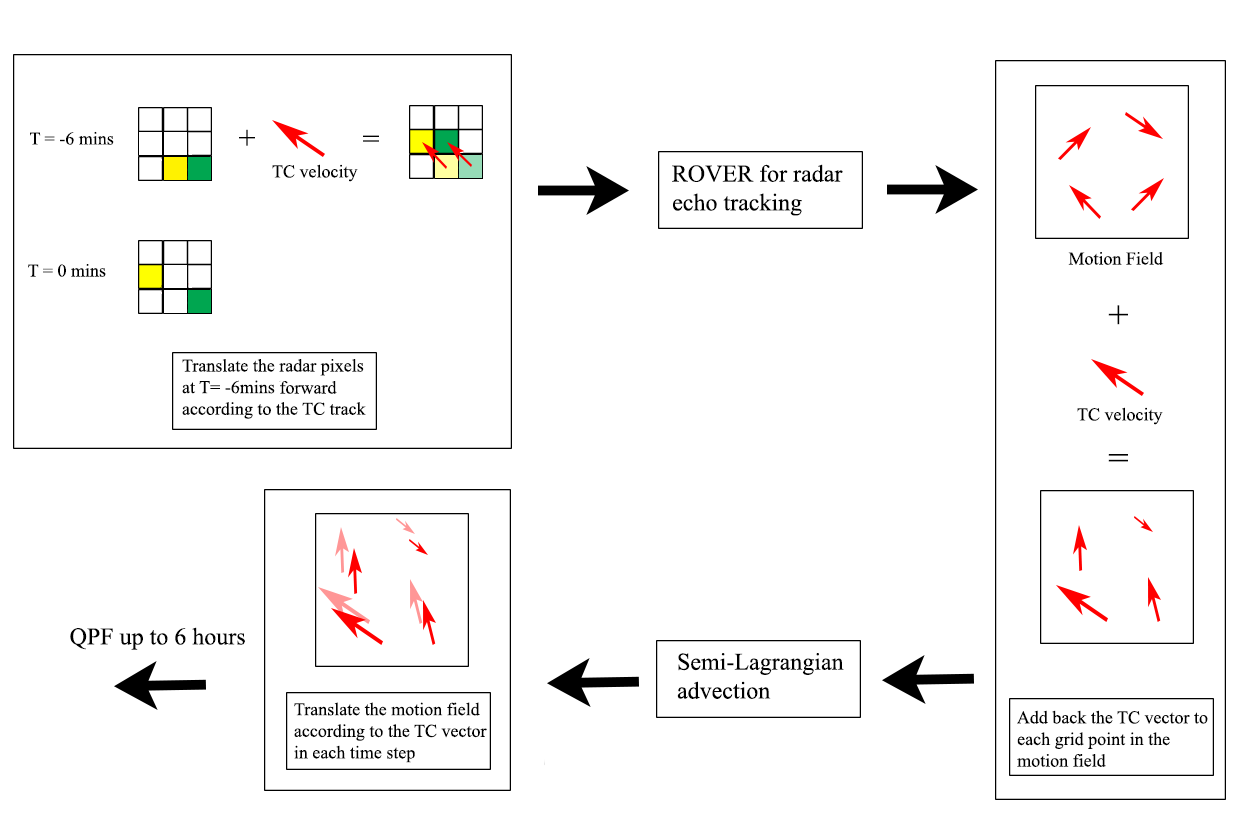
An illustration on the workflow of the steps taken in the Enhanced Scheme
Reference: W.C. Woo, K.K. Li, Michael Bala, 2014: An Algorithm to Enhance Nowcast of Rainfall Brought by Tropical Cyclones Through Separation of Motions. Tropical Cyclone Research and Review, 3(2), 111-121.
|